Protein-Ligand Binding Site Prediction
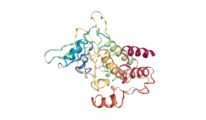
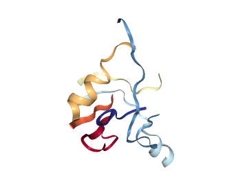
Predicting the binding site of a ligand on a protein is a crucial step in drug discovery. This project aims to predict the binding site of a ligand on a protein using a segmentation based deep learning model.
Introduction
Inferring knowledge from highly complex and high-dimensional data has always been a challenge in biology. Recently, deep-learning algorithms have taken the world by storm, achieving state-of-the-art results in various tasks like image classification, speech recognition, language translation and object detection. Deep learning algorithms take in raw inputs defined with a set of features and give predictions for the given task based on patterns buried inside. These algorithms perform exceptionally well with a massive amount of data. Since biology is a data-rich field with complex and unstructured data, scientists can apply deep learning for almost all tasks related to biology, potentially revolutionising this field. Deep learning approaches have already improved over previous scores achieved using traditional methods in specific tasks, although the gains in some studies are modest. This method can answer a biological or medical question, identifying essential features and predicting outcomes by harnessing heterogeneity across several dimensions of natural variation. Computer-aided drug design aims to make the drug discovery process faster and cheaper. Current research focuses more on the docking and scoring part of the drug discovery pipeline. However, these methodologies already assume that the protein’s binding site is already determined with high confidence. Accurate binding site detection is complex, and current methods are lacking in locating the druggable binding sites with high accuracy.
Traditional Approaches
Traditional approaches for binding cavity detection are typically geometry-based, but there are also examples of tools using binding energy to different chemical probes, sequence conservation (template or evolutionary methods) or a combination of these. For example, the ProBiS![]()
![]() ). Other approaches rely on a two-step algorithm, in which potential pockets are first identified and then scored to select the most probable binding sites. For example, Fpocket
). Other approaches rely on a two-step algorithm, in which potential pockets are first identified and then scored to select the most probable binding sites. For example, Fpocket
Methodology
The scPDB database
The 18 features used to describe an atom are:
- 9 bits (one-hot or all null) encoding atom types: B, C, N, O, P, S, Se, halogen and metal
- 1 integer (1, 2, or 3) with atom hybridization: hyb
- 1 integer counting the numbers of bonds with other heavy atoms: heavy_valence
- 1 integer counting the numbers of bonds with other heteroatoms: hetero_valence
- 5 bits (1 if present) encoding properties defined with SMARTS patterns: hydrophobic, aromatic, acceptor, donor and ring
- 1 float with partial charge: partialcharge
The output grid was also of the same size, centre and resolution but with binary masks for the presence of site atoms instead of atomic features. The output grid was converted to 3D probability densities for loss calculation. The input grid was of the shape (18,36,36,36) while the output grid was of the shape (1,36,36,36).
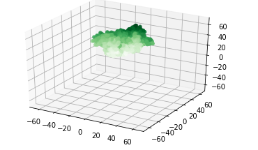
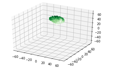
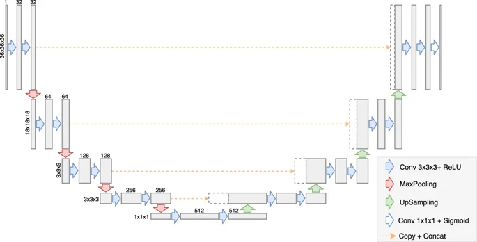
Deep learning model used is similar to the U-net architecture modified for the binding site prediction task. The model contains an encoder and a decoder network where the encoder compresses the input representation into a latent space and the decoder makes predictions based on the latent space which can localize features for highly accurate predictions. The model was developed using the PyTorch framework containing 4 encoder and 4 decoder blocks with one convolutional block in the bottleneck latent space. All the 2D blocks used in the original U-net architecture were modified to 3D blocks as the input was a 3D grid. Each block consists of two convolutional layers with the same number of filters (32, 64, 128, 256, or 512), kernel size of 3×3×3 pixels and ReLU activation function, combined either with a max-pooling layer or with an up-sampling layer. The two first max-pooling layers and the two last up-sampling layers have 2×2×2 patch sizes, while layers in the middle have 3x3x3 patch sizes. The feature maps in the middle of the network have spatial sizes of 1×1×1 and can be used as feature vectors. The model was trained with a batch size of 32 for 100 epochs after which the dice loss didn’t converge. Dice loss was used as the loss function for backpropagation of the neural network. Discretized volume overlap (DVO) was used as the metric for evaluation which is used to determine whether the predicted site is similar to the binding site or not. The dataset was split into a training and test set and the model achieved a DVO score of 0.623 on the test set.
Conclusion
The inference can be done using a CPU and enables fast detection of single or multiple binding sites in just under 10 seconds. Deep learning methods gained popularity in recent years because of their flexibility and potential for capturing complex relationships hidden in the data. Therefore, this work can also be seen as an example of adapting deep learning methods developed in other fields to structural bioinformatics.